1.8 Resize
Home and Learn - Free Excel VBA Course
11.3 Adding Charts to an Excel VBA User Form
In this tutorial, you'll learn how to add a chart to a user form. What we'll do is to have a dropdown list at the top of a form. When you select an option from the list, a chart will appear based on data from a spreadsheet.
Unfortunately, you can't just embed a chart onto a form like you can with a spreadsheet. You need to create an image of the chart you want and then load it into a picture box. The first thing to do, though, is to design the User Form.
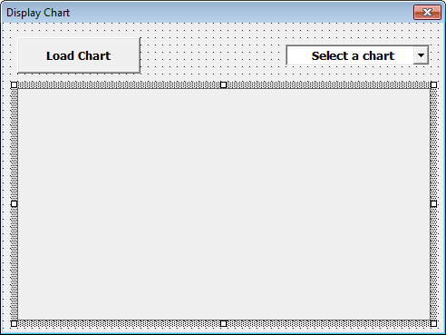
Start a new spreadsheet for this. Open up the Visual Basic Editor. From the menus at the top of the Editor, click Insert > User Form. You should see a grey form appear. With the form selected, locate the toolbox (View > Toolbox). Add a Command button to the top left of the form. Type Load Chart as the Caption property. Change the Name property to cmdLoad.
Now locate and select the Combo Box item in the Toolbox:

Draw one out in the top right of your form. Set the Text property to Select a Chart.
Now locate and select the Image control:

Draw an Image Box the size of the rest of your form. The whole of your form will then look like this:
With the design of the form out of the way, let's add the data to the spreadsheet.
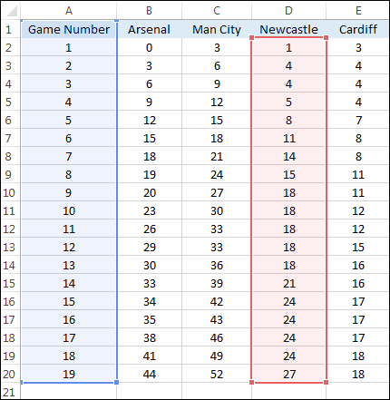
Return to Excel. Create a spreadsheet like the following:

The data is just some running points total for four football teams in the English premiership (season 2013 to 2014, when Cardiff and Newcastle United were in the Premiership). If you like, you can download a CSV file of the data here:
To import the data, click inside cell A1 on your spreadsheet. Then click on the Data ribbon at the top of Excel. Locate the Get External Data panel then click the From Text item. You'll then get a dialogue box where you can select the CSV file you downloaded above. A Text Import Wizard will appear to guide you the rest of the way. On step two of the Text Import Wizard, uncheck Tab as the delimiter and select Comma instead. Leave the other steps of the Wizard on the defaults. When you're done, you should have the data that you need for the rest of the tutorial.
Loading the Combo Box
We can use the Initialize event of forms to load the combo box with data. The data will be the team names in cells B1 to E1 on our spreadsheet. When a team is selected, a chart will appear in the Image box displaying the data for that team.
Go back to the coding window and your form. Double click your Command button
to get at its code. You should see your cursor flashing away in the Click event
of cmdLoad. We'll need to code here later. To get at the Initialize event,
have a look just above Private Sub cmdLoad_Click. You'll see a dropdown
list. From the list, select UserForm.

From the dropdown list just to the right of the UserForm one, select Initialize:

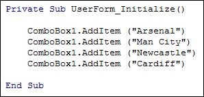
Private Sub UserForm_Initialize( )
End Sub
(A code stub for the UserForm_Click event may also be created. You can delete this.)To preload a combo box with text, you need to add items. You do this with the AddItem method of Combo boxes. Here's the first line for you Initialize event:
ComboBox1.AddItem ("Arsenal")
In between the round brackets of AddItem, you type whatever it is you want as text for the dropdown list. Enclose this between double quotes.
Add three more items:
ComboBox1.AddItem ("Man City")
ComboBox1.AddItem ("Newcastle")
ComboBox1.AddItem ("Cardiff")
Your code will then look like this
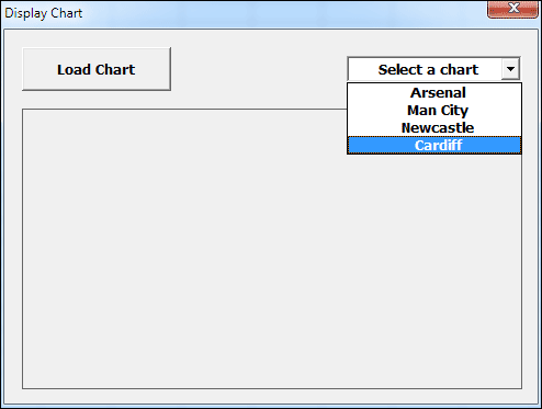
You can run your form to test it. Press F5 on your keyboard, or click Run > Run Sub User Form from the menu at the top of the Visual Basic Editor. Expand the drop down list and it should look like this: (we centred our list text with the TextAlign property.)
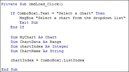
Stop your form from running and return to the Visual Basic Editor. In the code window, locate the cmdLoad_Click event code stub you got when double clicking your command button. The first thing we can do here is some error checking. We'll check to see if the dropdown list was left on the default "Select a chart". If it was, we can bail out. Add this code, then:
If ComboBox1.Text = "Select a chart" Then
MsgBox "Select a chart from the dropdown list"
Exit Sub
End If
We're using the Text property of Combo boxes and checking if this text reads "Select a chart". If it does, we display a message box and then Exit the Sub. That way, the rest of the code won't get executed.
For the next four lines, set up some variables:
Dim MyChart As Chart
Dim ChartData As Range
Dim chartIndex As Integer
Dim ChartName As String
We're setting up a Chart variable, a Range variable to hold the data from cells on the spreadsheet, an Integer variable to hold a value returned from the combo box, and a String variable for the name of the chart (this will appear at the top of the chart).
The next line to add is for grabbing that value from the combo box. It's this:
chartIndex = ComboBox1.ListIndex
The ListIndex property tells you which of the items from your list was selected. The first item in your list is at position 0, the next item at position 1, and so on.
Your code so far should look like this:
Once we have which item was selected from the combo box, we can use a Select Case statement to set the data from the spreadsheet. We can use ActiveSheet.Range for this:
Set ChartData = ActiveSheet.Range("B2:B20")
The ChartData variable will then contain a column of data from the spreadsheet.
We can also add a chart name:
ChartName = ActiveSheet.Range("B1")
We want the headings at the top, the team names. These are in cells B1, C1, D1 and E1.
Here's the Select Case statement to add to your code:
Select Case chartIndex
Case 0
Set ChartData = ActiveSheet.Range("B2:B20")
ChartName = ActiveSheet.Range("B1")
Case 1
Set ChartData = ActiveSheet.Range("C2:C20")
ChartName = ActiveSheet.Range("C1")
Case 2
Set ChartData = ActiveSheet.Range("D2:D20")
ChartName = ActiveSheet.Range("D1")
Case 3
Set ChartData = ActiveSheet.Range("E2:E20")
ChartName = ActiveSheet.Range("E1")
End Select
So if the chartIndex variable contains a 0 (the first item in the combo box) then the range B1:B20 from the spreadsheet will end up in the ChartData variable. The chart name will be taken from cell B1. But if the user selects the second item in the combo box then chartIndex will be 1, in which case the data from the range C1:C20 will end up in the ChartData variable. The chart name will be taken from cell C1. We continue like this for Case 2 and Case 3.
Your code should now look like this:

The next line to add is this rather curious one:
Application.ScreenUpdating = False
What this does is to turn off something called ScreenUpdating. This has two effects: one, it makes the code run faster; and two, it hides what Excel is doing. Our code will add a chart to the spreadsheet. But we only need to turn this chart into an image - we don't need to see it on screen. Once we have the chart as an image, we can delete it from the spreadsheet. We'll then turn ScreenUpdating back on later in the code.
For the next line, we can add a chart:
Set MyChart = ActiveSheet.Shapes. AddChart(xlXYScatterLines).Chart
Here, we setting the chart to be an XY Scatter Line one.
The problem we have now is that, expect for columns A and B, the data we want to use for the X axis and Y axis are not in adjacent columns. We want the X axis (the bottom one) to be the consecutive numbers in the A column (cells A2 to A20). We want this for all the charts. For the Y axis, we want the values from the B, C, D or E columns. Column B is OK because you're just selecting data like this in the spreadsheet below:

Excel will automatically use the A column for the X Axis. This is because it's adjacent to the B column, the Y axis.
But if want, say, the Newcastle chart, then we need to select data like this:
These two columns are not adjacent, so Excel doesn't know what to use for the X and Y Axes.
To select data the way we want it, we can use two properties of the SeriesCollection: Values and XValues. You use them like this:
MyChart.SeriesCollection(1).Values = ChartData
MyChart.SeriesCollection(1).XValues = ActiveSheet.Range("A2:A20")
Type a dot after SeriesCollection(1) and then type Values. After an equal sign, type the range of data you want to use as the values for this series. These values will then be used for the Y axis. For us, this is our range data that we stored in the ChartData variable. For the XValues, we want the range of values in cells A2 to A2.
Here's some code to add:
MyChart.SeriesCollection.NewSeries
MyChart.SeriesCollection(1).Name = ChartName
MyChart.SeriesCollection(1).Values = ChartData
MyChart.SeriesCollection(1).XValues = ActiveSheet.Range("A2:A20")
Notice the first two line. First we add a new series to the collection:
MyChart.SeriesCollection.NewSeries
Then we add the chart name:
MyChart.SeriesCollection(1).Name = ChartName
Whatever is in the variable ChartName will be used as the Name
property of SeriesCollection(1).
In the next lesson, you'll learn how to create an image of the chart using VBA code. We'll then place the image into the Image Box on the User Form.
Next Lesson: 11.4 Chart Images >