Home and Learn - Free Excel VBA Course
1.5 The VBA Developer Toolbar
Start a new spreadsheet for this. Now click on your Developer toolbar at the top of Excel. You should see this:

The above image is taken from Excel 2013 (Later versions of Excel are very similar). If you have an earlier version, you may not have the Add-Ins and Modify panels. But that's OK because we won't be using these.
The first panel to explore is the one on the left - Code:

There are five items on the Code panel: Visual Basic, Macros, Record Macro, Use Relative References, and Macro Security. You've already seen the Macro Security item. If you can't run your Macros then click this item and change the security settings.
Clicking the Visual Basic item opens up the Visual Basic editor. You can also press ALT + F11 on your keyboard as a shortcut.
Clicking the Macros item on the Code panel brings up the following dialogue box:

Once you create a few Macros, they will appear in the list. You can then run them by selecting a Macro Name and clicking the Run button.
The other two items are Record Macro and Use Relative References. We'll skip over these two, as we won't have too much use for them.
The panel we'll use a lot, though, is the Controls panel. It looks like this:

The first item, Insert, is expanded when you click on it. Doing so will reveal the following:

These are all the controls you can add to an Excel spreadsheet or a user form. We'll be adding one of these controls to a spreadsheet shortly. But back to the Controls panel. The other items are:
The Design Mode item is used to edit a control on a spreadsheet.
The Properties item shows you properties for a selected control.
The View Code item takes you to the Visual Basic editor again.
The Run Dialog item can be ignored, as we won't be using it.
We'll now create a Macro that selects a range of cells. These cells will be selected when we click a button on a spreadsheet.
To create the Macro, click the Visual Basic item on the Code panel. The Visual Basic Editor will open up. We want this Macro to be only for Sheet1 in the current Workbook. On the left hand side of the Editor, locate the Project Explorer panel. (If you can't see it, Click View > Project Explorer from the menu at the top of the Editor.)
In the Project Explorer right click the Sheet1 item under VBAProject (Book1):

From the menu that appears, select View Code. A blank coding window will open up. (You can also double click on Sheet1 to open up the code window.)
What we want to do here is to create a Subroutine. This Subroutine will be our Macro. Type the following line into the white coding area:
Sub Range_A1_D6()
Press the Enter key on your keyboard and the Editor should add the corresponding End Sub for you. Your coding window will then look like this:

So we now have a Subroutine (a Macro) with the name Range_A1_D6. In between Sub and End Sub enter the following code:
Range("A1:D6").Select
Your coding window should then look like this:

As you can guess, this code selects a range of cells. It selects the cells A1 to D6.
Before we try it out, you need to save your work.
From the menu bar at the top of the Editor, click File > Save Book1. The Save As dialogue box should appear. Change the name of the file to Range_Exercises.xlxs. Click the Save button and you should see an error message appear. This one:

Click No to return to the Save As dialogue box.
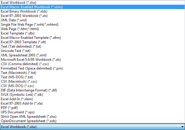
You get the error message because your file contains Macros. Excel can't save Macros in a file that end in xlxs. You need to change the file ending. To do that, click the Save As Type dropdown list. From the list, select Excel Macro-Enabled Workbook(*.xlsm):

Click the Save button again. When you click the Save button this time, the file should save OK. But note that the file ending is now xlsm.
Now that you know how to save a spreadsheet with a Macro in it, it's time to do something with that Macro. We'll add a button to a spreadsheet and activate our Sub when the button is clicked. We'll do that in the next part of this lesson below.
Next Lesson: 1.6 Spreadsheets Buttons >