Home and Learn - Free Excel VBA Course
1.6 Adding Buttons to an Excel Spreadsheet
In the previous lesson, you created a simple Sub in the code window. In this lesson, you'll activate that Sub from a button on a spreasheet.
At the top of the VBA Editor, locate the Excel icon, just under the File menu:
![]()
Click this icon to return to your spreadsheet. We'll now place a button control on the spreadsheet.
Locate the Controls panel on the Developer toolbar, and then click the Insert item. From the Insert menu, click the first item, which is a button:

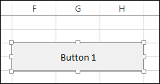
Now move your mouse to your spreadsheet. Hold down your left mouse button somewhere on the F column (F3 will do). Keep it held down and draw out a rectangular button. Let go of the left mouse button when your cursor is on H4
As soon as you let go of the left mouse button you'll see the Assign Macro dialogue box appear:

Select your Macro from the list and click OK. The button on your spreadsheet should now look like this:
You can edit the text on a button quite easily. Right click the button to see a menu appear. From the menu, select Edit Text:

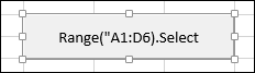
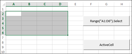
When you select Edit Text, a cursor will appear at the start of the text. Use the arrow keys on your keyboard to move the cursor to the end of the line. Delete the text Button 1 and type Range("A1:D6").Select instead (If you accidentally click away from the button, click on it again with right mouse button and not the left button. This will select your button again.):
Click away from the button to exit edit mode and you'll see the sizing handles disappear.
You can now test your button out. Give it a click and you'll see the cells A1 to D6 highlighted:

Congratulations! You have now written Excel VBA code to select a range of cells on a spreadsheet. And all with the click of a button!
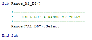
Now return to the Visual Basic editor (From the Developer toolbar, click Visual Basic on the Code panel.) Type a single quote before your Range line. The line should turn green:

The reason it turns green is because a single quote is used for comments. When the line is commented out it means Visual Basic will no longer see it as code, so doesn't do anything with it. You can add comments to remind yourself what your code does, as in the image below:
Adding comments to your code is a good habit to get in to. Especially when you come back to your code after a few weeks or so. If you haven't added comments you may not quite understand what it was you were trying to do.
Back to the Range code, though. Notice how we referred to the range of cells A1 to D6:
Range("A1:D6")
Another way to refer to the same range is like this:
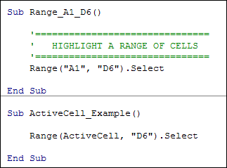
Range("A1", "D6").Select
This time, the start cell A1 and the end cell D6 are enclosed with double quotes. In between the two we have a comma.
Both the examples above do the same thing: they first select the top left cell of the range, and then the bottom right cell of the range. It's entirely up to you which you use. But with the second version you can use something called the ActiveCell.
ActiveCell
Instead of typing the name of a cell you can also refer to which cell on your spreadsheet is currently highlighted. The currently highlighted cell is called the ActiveCell (no spaces and with capital letters for the "A" and "C"). You can use this in your code. Let's see how it works.
After the End Sub of your first Subroutine, add the following:
Sub ActiveCell_Example()
Press the enter key on your keyboard to let the VB editor add the End Sub for you. Now add the following line between the Sub and End Sub of your code:
Range(ActiveCell, "D6").Select
Your coding window will then look like this:
So the top left cell we want to select is the ActiveCell, which is whatever cell you clicked in on your spreadsheet. The bottom right cell we want to select is D6.
Click the icon to return to your Excel spreadsheet. Now draw another button
on your form, just below the first one. You should see the Assign Macro dialogue
box appear again:

Select your new Macro (your Sub) from the list and click OK.
When you get back to your spreadsheet, edit the text of the button again. Type ActiveCell as the text. When you have finished editing the text, click away. Click inside another cell on your spreadsheet, cell A2 for example. Now click your button. You should see the cells A2 to D6 highlighted:
Click inside any other cell on your spreadsheet and click the button again. The cells from your active cell to D6 will be selected.
In the next part of this tutorial, we'll take a look at the Offset property. So save you work before moving on.
Next Lesson: 1.7 The Offset Property >